Binary Operations
Image processing has many applications. One of the significant applications of this is in medicine. Biomedical imaging is very important in diagnosis of serious illness such as cancer, malaria etc. For diagnosis of these diseases, the medical images must have a good distinction between the background and region of interest.[1] The reason for this is that the noisy background may cause one to make a wrong diagnosis.
There are methods in image processing that helps eliminate unwanted noise in the image. Morphological operations are used to clean the image from the noise. Combining the two techniques erosion and dilation would help us attain a cleaner image. The two operators that do this are the closing and opening operator. These operators are usually applied on binary images. An opening operator is a process in which an erosion is applied and then dilation with the use of the same structuring elements for both.[2] A closing operator is just the reverse of the opening operator. A closing operator is a process in which a dilation is applied and then erosion with the use of the same structuring elements for both. [3]
In this activity, we would perform operations that can be used in cancer cell screening. Cancerous cell are known to be larger than normal cells. This difference in size would help us determine which cells are cancerous. Here we would use all of the things we learned so far and the new morphological operators.
Here we have a photo which is similar to the image of human cells.
 |
| Figure 1. An image that is similar to photo of human cells |
 |
| Figure 2. A 256 x 256 pixel sub-image of the binarized image of figure 1. |
 |
| Figure 3. A code in Scilab when thresholding and converting to a binary image |
 |
| Figure 4. Image of the 12 sub-images when figure 1 is converted to a binary image. |
This photo was converted into a binary image and then divided to 12 subimages with dimension 256 x 256 pixels using gimp (see figure 2 and 4). I used Scilab with the code(see figure 3) shown below to convert it into a binary image and set the threshold that would give the best quality of the image. The threshold was set to 0.84. The 12 images have slight overlap with each other.
 |
| Figure 5. Scilab code using the opening and closing operator. |
To clean the image from the noises we used the opening and closing operators on each sub images. The structuring element I used was a circle with a size smaller to a single circle from the image but bigger than the ‘noise dots’ in the image. This was done using scilab(see figure 5).
After applying the operator this is one of the example of a subimage that was cleaned.

Figure 6. A sub-image that was cleaned using morphological operations
Then we recombine them and this was the result.
 |
| Figure 7. The recombined image of he cleaned subimages. |
To calculate for the best estimate of the area of the cells(blob), we used this command in Scilab(figure 8) and use this for all the subimages.
 |
| Figure 8. A code in Scilab to measure the area of the blobs |
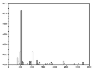
There is a small problem here since some of the cells’ areas overlap. To eliminate this problem, we look into the histogram plot of the areas measured. Then we find the range in which we are sure that there is no overlap(see figure 9).
 |
| Figure 9. The histogram plot of the measure areas of the cells(blobs). |
 |
| Figure 10. A single cell(blob) whose area is free of overlap. |
The range we used was 450-600 pixel count. To be sure, we measure a cell(blob) whose area is free of overlap(see figure 10). Here we get a result of 536 pixel count. This falls under the range chosen. After choosing the range we get the best estimate area for the blob using the command stdev in Scilab. What we got was 531.33 +/- 23.92. (note: the area measure for the single cell falls into this range).
Next we are given a photo similar to a photo of human cells with cancer cells.
 |
| Figure 11. Image of human cells(blobs) with some cells significantly bigger than others. |
We do the same things we did on the image in figure 1. After doing all these steps (binarizing, dividing, finding best estimate area), we find the cells that don’t fall on the best estimate area of a normal cell. To do this we use a circle as a structuring element and set its radius to ((mean area + uncertainty)/n)^0.5. by doing this the normal cells will be treated as noise when we perform the opening and closing operators on the image.
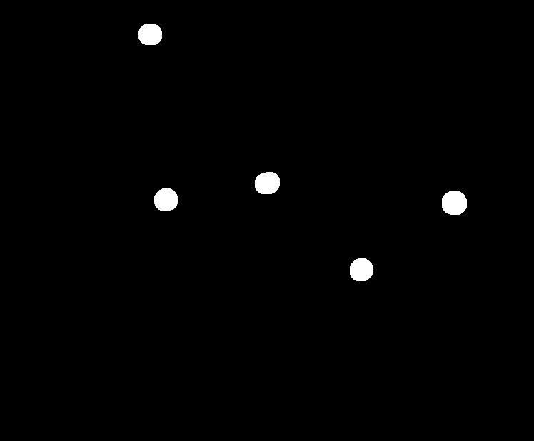 |
| Figure 12 . The cancer cells isolated using morphological operations. |
This would leave us with only the ‘cancer cells’ present.
References:
[2] Opening, http://homepages.inf.ed.ac.uk/rbf/HIPR2/open.htm
[3] Closing, http://homepages.inf.ed.ac.uk/rbf/HIPR2/close.htm