Activity 4

Area Estimation for Images with Defined Edges  

Measuring the area from an image has a lot of significance in medicine, industry and geography. Some of the applications of this are the detection of cancer cells in humans, quality inspection in electronic manufacture and land area estimation. Finding the area of a regularly shaped object is fairly easy since their formulas are known but irregularly shaped objects are the tricky ones. In reality we encounter irregular shaped objects more than regulary shaped ones. Techniques have been developed to calculate the area of images. Two of these techniques are the Green theorem and morphological operations. Morphological operations is a technique which needs pixel counting in blobs.

I made a square, equilateral triangle and circle using paint. I made the background black for all the shapes.

The images are shown below.  I used the Scilab and loaded the SIP toolbox to aid me in calculating the area of the shapes. I used the code below to see if the follow command really gets the edge pixel coordinates of the shape. 

Figure 1. Plot in Scilab of the edge pixel coordinates of the image of the circle below 

Figure 2. Image of a circle generated using Paint

  Figure 3. Plot in Scilab of the edge pixel coordinates of the image of the square below  

  Figure 4. Image of a square generated using Paint  

  Figure 5. Plot in Scilab of the edge pixel coordinates of the image of the triangle below  

  Figure 6. Image of a triangle generated using Paint  

Here is the code I used for this activity.

  

Lines 1 to 3 were used to get the pixel coordinate of the edge of the shapes. Lines 4 to 10 were used to calculate the area of the image using the Green’s theorem. Lines 11 to 14 were used to find the accuracy of the method. Below are the data obtained for the three shapes:

Shape	Calculated Value	Analytic Value	Accuracy
Triangle	18038.5	18324	98.441934
Circle	29675	30004	98.90348
Square	37681.5	38220	98.591052

Figure 7. Image of the Quezon Hall in google map 

Figure 8. Image of the Quezon Hall masked in Adobe Photoshop

Figure 9. The Background of the area was set to black

  Figure 10. Plot in Scilab of the edge pixel coordinates of the image of Quezon Hall 

Area of Quezon Hall

Calculated value = 1976

Analytic value =  2118

Accuracy =  

I would give myself a grade of 10 for this activity for being able to do all the requirements and explaining it well. I enjoy learning something new so I enjoyed this activity.

Image Types and Formats

Activity 3

Image Types and Formats

We live in a visual world. Almost everyone has a digital camera and try to capture every significant moment in their lives. These digital images are then downloaded or uploaded to the web. Digital images are also used to share information. With the importance of the digital images, basic information on them is necessary these days. To know what format to use to preserve the quality of the image or to decrease the size of the image without sacrificing its quality. It is also important to know what type of image would one need to capture an information.

A. Image Types

There are a lot of type of digital images. Here are the the basic types of digital images:

(Note:To view the properties of the images using scilab; use this code

iminfo(<filename>, 'verbose'>))

1. Indexed Image: These images cantains two sets of data: one for the image and the other for the colormap. These images eats up less space on your hard disk but may be have lower quality.

Figure 1. An example of an indexed image.

File Name: stock-photo-fingerprint-over-background-of-binary-numbers-56638072.jpg

File Size:   53,604 bytes

Height: 388 rows

Width: 450

Bit  depth: 8

DPI: 300

Color Type: Grayscale

Source: http://www.shutterstock.com/pic-56638072/stock-photo-fingerprint-over-background-of-binary-numbers.html

2. Binary Image   :These images are composed of pixels containing values of either 0 or 1. These type of image are often used in images where we seek to see only the line shape information. Examples of these re fingerprints and signature. 

Figure 2. An Example of a Binary Image

File Name: signat.png

File Size: 3,115 bytes

Height: 125

Width: 400

Bit  depth: 24

Color Type: Grayscale

Source: http://www.forum.arcadetrainer.com/viewtopic.php?f=8&t=16694

3. Grayscale image:These image type differ from binary image since its gray levels range from black to white in fine steps.

Figure 3. An Example of a grayscale image

File Name: 722999-3436-x-rays-7-mri-scans.jpeg

File Size: 2,595 bytes

Height: 144

Width: 108

Bit  depth: 24

Color Type: Grayscale

DPI: 72

Source: http://www.fotolibra.com/gallery/699562/x-ray/like/

4. Truecolor image: These images are composed of set of pixels with values for red, green and blue. Each specific area has a designated pixel color information.

Figure 4. An example of a truecolor image

File Name: zspic.jpg

File Size: 79,266 bytes

Height: 482

Width: 720

Bit  depth: 24

Color Type: truecolor

DPI: 72

Source: personal photo

5. High Dynamic Range :There are things that need more than 8-bit grayscale to understand. This is where HDR images are needed.

Figure 5. An example of a high dynamic range image

File Name: hdr-76.jpg pic.jpg

File Size: 21,835 bytes

Height: 301

Width: 450

Bit  depth: 24

Color Type: truecolor

DPI: 96

Source: www.smashingmagazine.com/.../35-fantastic-hdr-pictures/

6. Multi or hyperspectral image Unlike other image types, multispectral image has more than three bands, it has bands in the order of 10.

Figure 6. An example of a hyperspectral image

Source:http://en.wikipedia.org/wiki/Hyperspectral_imaging

7. 3D images This image type stores spatial 3D information.
 

Figure 7. An example of a 3D image

8. Temporal images or Videos. Capturing videos now had been more advance than before. We are now able to capture motion in high definition.

An example of a digital video

B. File format

Lossless compression compresses the data without compromising the quality of the image. Data are compressed by finding similar pixels in the image. Lossy compression, compresses the data even if it results in an image with lower resolution. This depends on the limitation of the human eye to detect the change. 

BMP (bitmap) 

 (1 to 32-bit color depth.) 

These type supports indexed colors and has various color depths.

Figure 8. An example of an image with a BMP format

GIF (Graphics Interchange Format) 

 (1 to 8-bit color depth)

This also supports indexed color and animation. This is used in the web and there are no details lost when you save it in this format. It is a lossless compression.

Figure 9. An example of an image with a GIF format

JPEG (Joint Photographic Experts Group) 

(8, 12, 24-bit color depth)

This format has issues when saving an image with a text. This has a lossy compression and details are lost when you save the image.

Figure 10. An example of an image with a JPG format

PNG (Portable Network Graphics) 
(1, 2, 4, 8, 16, 24, 32, 48, 64-bit color depth)

This format supports transparencies and is good for making the file size small without loss in detail. This is done by looking at patterns of pixel in the image. This is good for text since it prevents anti-aliasing in text. It has a lossless compression.

Figure 11. An example of an image with a PNG format

TIFF (Tagged Image File Format) 

This format is good for huge images with a very high resolution. These are images needed for huge billboard ads and posters. It has a lossless compression and no data is lost when you save it.

(1, 2, 4, 8, 16, 24, 32-bit color depth) 

C. Working with Images in Scilab

In these part we would look in to the basic things you can do in Scilab with your images. 

Figure 12. The truecolor image that would be edited

The first thing I did was convert the truecolor image above to a binary type. The result is the figure below.

Figure 13. A binary image derived by converting a truecolor image  to binary using Scilab

This was done by using the code below in Scilab. 

The next thing I did was convert the truecolor image to a grayscale one. The resulting image is shown below.

Figure 14. A grayscale image derived by converting a truecolor image  to grayscale using Scilab

This was done by using the code below in Scilab.

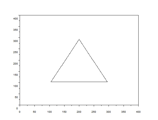
The next thing I did was work on the image of the hand drawn graph from activity 1. 

Figure 15. The hand drawn graph from activity 1

I looked into the graylevel histogram of the grayscaled image. to do this I used the following code below in Scilab. Histograms may be used to effectively determine what threshold of conversion to use in a certain image.  By looking at the histograms below of the graph, I selected the threshold 0.7. Notice the difference in quality of the two images. 

Figure 16. The histogram of the hand-drawn graph

Figure 17. The original hand-drawn graphs(left) and the graph after threshold 0.7 was chosen(right).

I would give myself a grade of 10 for being able to research well regarding this topic and presenting it nicely. Ienjoyed doing this and learned a lot on this topic regarding digital images.

[1] Soriano, M., 2011. Image types and formats. Applied Physics 186.

Scilab Basics-activity 2

Scilab is a programming language that makes it easy for one to deal with array and matrices. Its commands makes problems with matrices very easy to tackle. In this activity we were asked to make synthetic images to test algorithms and to see if we understood the basic commands in Scilab.

The first image that was made was a circle aperture. This was given as an example to us. The code is shown below.

Circle Aperture


[1] nx = 100; ny = 100; //defines the the number of elements along x and y
[2] x = linspace(-1,1,nx); //defines the range
[3] y = linspace(-1,1,ny);
[4] [X,Y] = ndgrid(x,y); //creates two 2D arrays with x and y coordinates
[5] r= sqrt(X.^2 + Y.^2); //note element-per-element squaring of X and Y
[6] A = zeros (nx,ny);
[7] A (find(r<0.7) ) = 1;
[8] imshow (A, []);

The image generated from this code is shown below.

Fig. 1 Image of the circle aperture generated using Scilab

I used lines 1 to 4 from the sample code to create the arrays for all of the images generated here.

Annulus

To create the annulus, I used the lines 1 to 6 from the code to generate the circle aperture. I then add lines 7 -11 below. This was done to generate an outer and inner circle for the annulus.

[7] ro = 0.8; //radius of outer circle

[8] ri = 0.4; //radius of inner circle

[9] A(find(r<ro)) = 1;

[10] A(find(r<ri)) = 0;

[11] imshow(A, []);

Fig. 2 Image of the annulus generated using Scilab

Circular aperture with graded transparency

To create the circular aperture with graded transparency, I once again used lines 1 to 6 from the code to generate the circle aperture. I add to the code lines 7-8 since I assumed a gaussian distribution for the beam and multiplied the matrix of the circular aperture with it. 

[7] G = exp(-4*X.^2 - 4*Y.^2); //gaussian multiply to matrix

[8] imshow(G,[]);

Fig. 3 Image of the circle aperture with graded transparency generated using Scilab

Centered square aperture


I added lines 5-8 to generate the aperture. The side was set to 0.3
[5] A = zeros(nx,ny);
[6] s = 0.3; //sets the length of a side
[7] A(find(abs(X) <s & abs(Y)<s))=1;
[8] imshow(A, []);

Fig. 4 Image of the centered square aperture generated using Scilab

Sinusoid along the x-direction (corrugated roof)


I added lines 5-10 tp set the amplitude and frequency for the sinusoid and restricted it to zero and positive values to generate the sinusoid.

[5] A = zeros(nx,ny);
[6] a = 3; //sets the amplitude of sinusoid
[7] f = 30; //sets the frequency of sinusoid
[8] A = a*sin(f*X);
[9] A = A + abs(min(A)); // restricts to non-negative values
[10] imshow(A, []);

Fig. 5 Image of the sinusoid along x-direction generated using Scilab

Grating along the x-direction 8 divisions

I add lines 5-10 to the code. What this does is divide the elements along x by 8 to produce a grating with 8 divisions.

[5] A = zeros(nx,ny);
[6] A(1:nx/8, 1:ny) = 1;
[7] A(2*nx/8:3*nx/8, 1:ny) = 1;
[8] A(4*nx/8:5*nx/8, 1:ny) = 1;
[9] A(6*nx/8:7*nx/8, 1:ny) = 1;
[10] imshow(A, []);

Fig. 6 Image of the grating generated using Scilab

For this activity, I would give myself a grade of 9/10. It was a little bit rushed so my presentation wasn't that great and very detailed but I did all the requirements. The image generated looked correct. I would like to thank Ma'am Soriano for the tip she gave me to make my scilab and sip toolbox work. I also looked at the Scilab hands on tutorial by satish annigeri.